Congratulations on your approved PARADIM proposal. This tutorial explains how to get access to the JHU-MARCC high-performance computing center with an approved PARADIM proposal. If you do not have an approved project and are interested in submitting a two-page proposal, please use the link: https://www.paradim.org/project proposals.
Running Jobs at Computational Facilities (pdf download)
This tutorial discusses, 1) how to submit jobs at JHU-MARCC with a sample job submission file, 2) how to run interactive jobs at JHU-MARCC, 3) useful commands related to job submission, 4) useful Linux commands, and 5) how to submit jobs at XSEDE with a sample job submission file.
1. How to Submit Jobs at JHU-MARCC
MARCC policy states that all users must submit jobs to the scheduler for processing. Interactive use of login nodes for job processing is not allowed.
MARCC uses,
SLURM resource manager to manage resource scheduling and job submission.
Partitions (different job queues) to divide types of jobs which will allow sequential/shared computing, parallel, GPU jobs, and large memory jobs.
For the complete list of partitions available for users please visit:
A sample script to run a Quantum Espresso job in parallel partition using 24 cores with 5000MB memory in a single node would look like this,
#!/bin/bash -l
#SBATCH --job-name= myjob-1
#SBATCH --time=00:30:00
#SBATCH --partition=parallel
#SBATCH --nodes=1
#SBATCH --ntasks-per-node=24
#SBATCH --mem-per-cpu=5000MB
mpirun -np 24 pw.x < silicon.in > silicon.out
Jobs are usually submitted via a script file. The sbatch command is used.
$ sbatch my-script
2. How to Run Interactive Jobs at JHU-MARCC
Users who need to interact with their codes while these are running can request an interactive session. This will submit a request to the queuing system that will allow interactive access to the node.
If you would like an interactive session, you can use the following command
$ interact -p parallel -n 24 -c 1 -t 60 -m 5G
Here we are requesting 24 CPUs, since -n 24 is the number of tasks, and -c 1 is the number of cores per task. We are asking for a session of 60 min (-t 60) and with a total memory of 5 GB (-m 5G).
This command opens a session where we will be able to execute pw.x directly from the command line without a job submission script.
$ mpirun -n 24 pw.x < silicon.in > silicon.out
3. Useful Commands for job Submission
$ sbatch my-script submit a job script
$ squeue list all jobs
$ sqme list all jobs belong to the current user
$ squeue -u [userid] list jobs by user
$ squeue [job-id] check job status
$ scancel [job-id] delete a job
$ scontrol hold hold a job
$ scontrol release release a held job
$ sacct show finished jobs
*Users can still use torque commands like qsub, qdel, qstat, etc…
find – search for files in a directory hierarchy Usage: find [OPTION] [path] [pattern] eg. find myscript.txt, find -name myscript.txt
history – prints recently used commands Usage: history
ps – report a snapshot of the current processes Usage: ps [OPTION] eg. ps, ps -el
kill – to kill a process Usage: kill [OPTION] pid eg. kill -9 2275
5. How to Submit Jobs at XSEDE
Allocation for The Extreme Science and Engineering Discovery Environment (XSEDE) is available for collaborative research only. Please contact members of PARADIM theory staff available at /people to get access to XSEDE allocations.
If you already have an allocation with XSEDE, following is a sample job scrip to submit jobs.
#!/bin/bash
#SBATCH -J myMPI # job name
#SBATCH -o myMPI.o%j # output and error file name (%j expands to jobID)
#SBATCH -n 32 # total number of mpi tasks requested
#SBATCH -p development # queue (partition) -- normal, development, etc.
#SBATCH -t 01:30:00 # run time (hh:mm:ss) - 1.5 hours
#SBATCH --mail-type=begin # email me when the job starts
#SBATCH --mail-type=end # email me when the job finishes
ibrun ./pw.x # run the MPI executable named pw.x
Quantum Espresso (QE) is an integrated suite of Open-Source computer codes for electronic-structure calculations and materials modeling. It is based on density-functional theory, plane waves, and pseudopotentials. In this set of tutorials, you will learn how to run the essential calculations based on density functional theory as implemented in QE on JHU-MARCC, a shared computing facility. You can practice running calculations in various listed topics starting with a test run.
QE is an Open Source distribution. The primary references of the QE code are the articles:
P. Giannozzi et al., J. Phys.: Condens. Matter21, 395502 (2009)
P. Giannozzi et al., J. Phys.: Condens. Matter29, 465901 (2017)
Test Run (pdf download)
In this tutorial we will prepare a simple job and execute it on JHU-MARCC. The goal is to make sure that we have configured Quantum Espresso properly and everything runs well. We will run a simple total energy calculation (scf calculation) for silicon in the diamond structure. We will also learn how to use the command line to create an input file and a job submission file to submit our job to the queue.
Convergence Parameters of DFT Calculations (pdf download)
In this tutorial we will explore two important convergence parameters of DFT calculations, the planewave kinetic energy cutoff ecutwfc, and the Brillouin zone sampling k-points. As an example, for silicon, we study how the total energy, the number of planewaves, and the timing vary as a function of the planewaves cutoff ecutwfc, and how the total energy of silicon varies with the number of k-points. As an exercise, we also explore the scaling of DFT calculations as a function of system size.
Equilibrium Structure of a Diatomic Molecule and a Bulk Crystal (pdf download)
Among all possible structures, the equilibrium structure at zero temperature and zero pressure is found by minimizing the DFT total energy. In this tutorial we will learn the concept of calculating the equilibrium structure. We will calculate 1) the equilibrium structure and the binding energy of a diatomic molecule using the Cl2 molecule as an example, 2) the equilibrium structure and the cohesive energy of a bulk crystal using silicon, and 3) the equilibrium lattice parameter of silicon, diamond, and graphite.
Automatic Optimization of Crystal Structure and Elastic Constant (pdf download)
In this tutorial we will 1) automatically optimize the atomic coordinates by using calculation type relax and 2) automatically optimize the unit cell by using calculation type vc-relax. We will then familiarize ourselves with calculation of bulk modulus and the elastic constant, using diamond as a test case. As an exercise, we will set up a new calculation on SrTiO3 starting with a simple input file for the material. To find the initial geometry for the unit cell and atomic coordinates, we search the Materials Project Database.
Phonon Dispersion (pdf download)
In this tutorial we will learn how to calculate 1) the vibrational frequencies of a diatomic molecule, Cl2, 2) phonon dispersion relations of diamond, GaAs, and SrTiO3, and 3) LO-TO splitting, IR activity, and low-frequency dielectric constants of a polar semiconductor, GaAs.
Band Structure and UV/VIS Spectra (pdf download)
In this tutorial we will explore how to 1) calculate the band structure and visualize the wavefunctions corresponding to selected Kohn-Sham eigenvalues of silicon, and 2) calculate the band structure and the corresponding optical absorption spectrum (UV/Vis spectra) of GaAs to obtain the imaginary part of the dielectric function, e2(ω), which is related to the optical absorption coefficient κ(ω).
YAMBO is a code for Many-Body calculations in solid state and molecular physics to accurately determine excited states. YAMBO relies on the Kohn-Sham wavefunctions generated by DFT codes such as Quantum Espresso (QE). In this set of tutorials, you will first learn how to configure YAMBO with QE on JHU-MARCC and then you can practice running a range of calculations covering various topics. Tutorials include ground state calculation, file conversion, quasiparticle GW band structure calculation, and the calculation of optical absorption spectra using the Bethe-Salpeter equation (BSE).
The YAMBO code was originally developed in the Condensed Matter Theoretical Group of the Physics Department at the University of Rome "Tor Vergata" by Andrea Marini.
The primary reference for YAMBO code is the article:
Yambo: an ab initio tool for excited state calculations, Andrea Marini, Conor Hogan, Myrta Grüning, Daniele Varsano, Comp. Phys. Comm.180, 1392 (2009).
Ground State Calculation as Starting Point for YAMBO (pdf download) The initial step is to generate the ground state wavefunction for the proposed system using Quantum Espresso. In this tutorial we are going to use single layer MoS2 as an example material for our QE ground state calculation. We discuss the specific input parameters used for both self-consistency (SCF) and non-self-consistency (NSCF) runs to obtain the ground state wavefunction, which we will then use for YAMBO calculations. Please go to the Quantum Espresso Tutorial if you need further information about QE.
File Conversion from QE to YAMBO (pdf download) In this tutorial we are going to learn how to convert QE-generated wavefunctions into YAMBO-readable format. These wavefunctions will be the basis for the calculation of excited states in the following step.
GW Band Structure (pdf download) DFT methods usually underestimate the band gap. In this tutorial we are going to learn how to calculate the quasiparticle correction to the band gap using the GW approximation implemented in YAMBO. We are going to use the command line to generate the input file for the GW calculation. We are also going to discuss the input parameters that require convergence tests during the GW calculation.
Postprocessing of the Quasiparticle Energies to Obtain the GW Band Structure (pdf download) Once the GW calculation is completed, we are going to use the yambo post-processor ypp, along with a set of commands, to plot the GW band structure.
Calculation of Optical Properties with YAMBO (pdf download) In this tutorial we are going to calculate the optical absorption spectrum using the GW-BSE method implemented in YAMBO. We are going to calculate the absorption spectrum including the quasiparticle correction for single layer MoS2. Before starting this tutorial, you must first complete the GW tutorial since this calculation depends on previously calculated corrected quasiparticle energies.
Tutorial: Working with Mismatched INterface Theory (MINT) and the 3D MINT-Sandwich Approach
Betül Pamuk, ORCID 0000-0002-2817-0592
Drake Alexander Niedzielski, ORCID 0000-0002-9607-8042
Eli Gerber, ORCID 0000-0002-9594-6450
Eun-Ah Kim, ORCID 0000-0002-9554-4443
Tomás Alberto Arias, ORCID 0000-0001-5880-0260
DOI: 10.34863/seqm-4p70
The Materials-by-Design approach relies on strong theoretical capabilities to predict the properties of novel materials. Interface quantum materials are the focus of PARADIM’s in-house research and many of these materials have a lattice mismatch between the two materials at the interface.
Traditional ab initio techniques for calculating the electronic structure of materials are powerless when the lattice mismatch between two crystals leads to the absence of periodicity. The two common approaches to dealing with aperiodic systems are the cluster approach and the supercell approach. In the former case, one builds a large, isolated-cluster of the periodic material to simulate a mostly periodic structure. In the latter case, one builds a large periodic supercell of the aperiodic structure to enable the application of high performance techniques developed for periodic systems. Unfortunately, in both cases, the simulations become computationally expensive and time consuming as the simulation size increases. Both methods assume a convergence toward the exact behavior as the simulated material size reaches infinity. This assumption depends on the “nearsightedness” of electronic matter.
To overcome this issue, Prof. Kim and Prof. Arias have developed Mismatched Interface Theory (MINT) to study incommensurate interfaces. MINT combines the supercell and cluster approaches directly within standard density functional theory (DFT). The nearsightedness of the electronic matter also ensures that the convergences are achieved rather rapidly with MINT.
This tutorial provides an example of a MINT calculation for the incommensurate Graphene/α-RuCl3 interface. For further explanation of the theory behind MINT as well as converged results, please refer to E. Gerber et al. Phys. Rev. Lett. 124, 106804 (2020).
The calculations in the tutorial are performed by JDFTx (http://jdftx.org/) code, but the MINT theory is general enough that it can be used with the charge density output of any DFT code.
This tutorial assumes that the user is familiar with DFT. If the user is not familiar with DFT, we recommend looking into our PARADIM summer school videos, PARADIM tutorials (based on a different code, Quantum Espresso) as well as tutorials on the JDFTx website to familiarize yourself with how DFT calculations work.
Substrate Material, α-RuCl3
We first start with a large periodic supercell of the substrate material, which is the material system of primary interest, α-RuCl3 in this example.
lattice \
22.5252 0  0\
0    19.5068 0\
0     0     35

kpoint-folding 6 4 1
ion-species /home/bpamuk/scr4_tmcquee2/betul/MINT/MINT_tutorial_files_Eli/RUNS/pseudos/Ru_ONCV_PBE-1.0.upf
ion-species /home/bpamuk/scr4_tmcquee2/betul/MINT/MINT_tutorial_files_Eli/RUNS/pseudos/Cl_ONCV_PBE-1.0.upf
elec-cutoff 30

elec-n-bands 197  # num of valence e in u.c./2. 4*16+12*7+30=178/u.c.
elec-smearing Fermi 0.003
electronic-minimize energyDiffThreshold 0.00005

dump-name Ru8C14dens.$VAR
Dump End ElecDensity State
Dump End IonicPositions
Dump End Lattice

coords-type Cartesian

ion Ru  0       0       0       0
ion Ru  11.26262072     0       0       0
ion Ru  -0.009694315    6.425327665     -0.000321254    0
ion Ru  11.25292641     6.425327665     -0.000321254    0
ion Ru  -5.635911855    9.73609683      0.008352607     0
ion Ru  5.62670887      9.73609683      0.008352607     0
ion Ru  -5.634041022    16.27378784     -0.01273678     0
ion Ru  5.628579702     16.27378784     -0.01273678     0
ion Cl  -1.731672983    3.23689962      2.608280935     0
ion Cl  9.530947742     3.23689962      2.608280935     0
ion Cl  -1.955719372    16.4294827      2.545088364     0
ion Cl  9.306901353     16.4294827      2.545088364     0
ion Cl  -7.597187033    -0.130126808    2.566839156     0
ion Cl  3.665433692     -0.130126808    2.566839156     0
ion Cl  -7.587511615    6.635352257     2.568332043     0
ion Cl  3.675109109     6.635352257     2.568332043     0
ion Cl  -1.949880106    9.571803704     2.539456969     0
ion Cl  9.312740618     9.571803704     2.539456969     0
ion Cl  -7.323818691    13.01566655     2.54266951      0
ion Cl  3.938802034     13.01566655     2.54266951      0
ion Cl  -9.526922617    3.241359383     -2.602214902    0
ion Cl  -9.316482284    16.43628572     -2.551229987    0
ion Cl  -3.657893669    -0.125402483    -2.569919416    0
ion Cl  1.735698108     3.241359383     -2.602214902    0
ion Cl  1.946157338     16.43628572     -2.551229987    0
ion Cl  7.604727055     -0.125402483    -2.569919416    0
ion Cl  -3.653868544    6.631308235     -2.549510332    0
ion Cl  1.940488148     9.560559811     -2.535242871    0
ion Cl  7.60875218      6.631308235     -2.549510332    0
ion Cl  -9.322132577    9.560559811     -2.535242871    0
ion Cl  -3.94106971     13.00948714     -2.54805524     0
ion Cl  7.321551015     13.00948714     -2.54805524     0

spintype z-spin
initial-magnetic-moments Ru 1 -1 -1 1 1 -1 -1 1 Cl 0 0 0 0 0 0 0 0 0 0 0 0 0 0 0 0 0 0 0 0 0 0 0 0
Cluster Material, Graphene Flake
Next, we create a cluster, a graphene flake in this example, such that the adjacent cluster images do not interact with each other. (Note that, in this example, we also terminate the edges of the flake with hydrogen atoms to eliminate dangling bonds and increase the rate of convergence with flake size.) Here is an example of a flake with 14 C sites:
lattice \
22.5252 0  0\
0    19.5068 0\
0     0     35
kpoint-folding 6 4 1
ion-species /home/bpamuk/scr4_tmcquee2/betul/MINT/MINT_tutorial_files_Eli/RUNS/pseudos/C_ONCV_PBE-1.0.upf
ion-species /home/bpamuk/scr4_tmcquee2/betul/MINT/MINT_tutorial_files_Eli/RUNS/pseudos/H_ONCV_PBE-1.0.upf

elec-cutoff 30

elec-n-bands 197  # num of valence e in u.c./2. 4*16+12*7+30=178/u.c.
elec-smearing Fermi 0.003

electronic-minimize energyDiffThreshold 0.00005

dump-name Ru8C14dens.$VAR
Dump End ElecDensity State
Dump End IonicPositions
Dump End Lattice
coords-type Cartesian
ion C   4.67050549      8.653759177     6.584456559867589       0
ion C   6.893392999     7.345691851     6.584456559867589       0
ion C   6.893392999     4.654308149     6.584456559867589       0
ion C   4.67050549      3.346240823     6.584456559867589       0
ion C   -4.67050549     3.346240823     6.584456559867589       0
ion C   -6.893392999    4.654308149     6.584456559867589       0
ion C   -6.893392999    7.345691851     6.584456559867589       0
ion C   -4.67050549     8.653759177     6.584456559867589       0
ion C   0       8.648964932     6.584456559867589       0
ion C   0       3.351035068     6.584456559867589       0
ion C   2.302773955     7.361204644     6.584456559867589       0
ion C   2.302773955     4.638795356     6.584456559867589       0
ion C   -2.302773955    4.638795356     6.584456559867589       0
ion C   -2.302773955    7.361204644     6.584456559867589       0
ion H   4.659683006     10.702098       6.584456559867589       0
ion H   8.678469751     8.345243747     6.584456559867589       0
ion H   8.678469751     3.654756253     6.584456559867589       0
ion H   4.659683006     1.297902004     6.584456559867589       0
ion H   -4.659683006    1.297902004     6.584456559867589       0
ion H   -8.678469751    3.654756253     6.584456559867589       0
ion H   -8.678469751    8.345243747     6.584456559867589       0
ion H   -4.659683006    10.702098       6.584456559867589       0
ion H   0       10.69934088     6.584456559867589       0
ion H   0       1.30065912      6.584456559867589       0

spintype z-spin
initial-magnetic-moments C 1 -1 1 -1 1 -1 1 -1 1 -1 1 -1 1 -1 H 0 0 0 0 0 0 0 0 0 0
MINT bilayer interface, Graphene/α-RuCl3
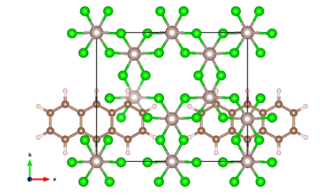
Next, we place the graphene flake on top of the substrate α-RuCl3 and relax the ionic coordinates:
Fig. 1 Top view of the Graphene/α-RuCl3 interface. Light brown atoms are Ru, green atoms are Cl, dark brown atoms are C, and light gray atoms are H. Note that the graphene is pacified by H atoms to avoid any dangling bonds.
lattice \
22.5252 0  0\
0    19.5068 0\
0     0     35

kpoint-folding 6 4 1

ion-species /home/bpamuk/scr4_tmcquee2/betul/MINT/MINT_tutorial_files_Eli/RUNS/pseudos/Ru_ONCV_PBE-1.0.upf
ion-species /home/bpamuk/scr4_tmcquee2/betul/MINT/MINT_tutorial_files_Eli/RUNS/pseudos/Cl_ONCV_PBE-1.0.upf
ion-species /home/bpamuk/scr4_tmcquee2/betul/MINT/MINT_tutorial_files_Eli/RUNS/pseudos/C_ONCV_PBE-1.0.upf
ion-species /home/bpamuk/scr4_tmcquee2/betul/MINT/MINT_tutorial_files_Eli/RUNS/pseudos/H_ONCV_PBE-1.0.upf

elec-cutoff 30

elec-n-bands 197  # num of valence e in u.c./2. 4*16+12*7+30=178/u.c.
elec-smearing Fermi 0.003
#lattice-minimize energyDiffThreshold 0.0001 nIterations 10
#ionic-minimize energyDiffTHreshold 0.0001 nIterations 10
electronic-minimize energyDiffThreshold 0.00005

dump-name Ru8C14dens.$VAR
Dump End ElecDensity State
Dump End IonicPositions
Dump End Lattice
coords-type Cartesian
ion C   4.67050549      8.653759177     6.584456559867589       0
ion C   6.893392999     7.345691851     6.584456559867589       0
ion C   6.893392999     4.654308149     6.584456559867589       0
ion C   4.67050549      3.346240823     6.584456559867589       0
ion C   -4.67050549     3.346240823     6.584456559867589       0
ion C   -6.893392999    4.654308149     6.584456559867589       0
ion C   -6.893392999    7.345691851     6.584456559867589       0
ion C   -4.67050549     8.653759177     6.584456559867589       0
ion C   0       8.648964932     6.584456559867589       0
ion C   0       3.351035068     6.584456559867589       0
ion C   2.302773955     7.361204644     6.584456559867589       0
ion C   2.302773955     4.638795356     6.584456559867589       0
ion C   -2.302773955    4.638795356     6.584456559867589       0
ion C   -2.302773955    7.361204644     6.584456559867589       0
ion H   4.659683006     10.702098       6.584456559867589       0
ion H   8.678469751     8.345243747     6.584456559867589       0
ion H   8.678469751     3.654756253     6.584456559867589       0
ion H   4.659683006     1.297902004     6.584456559867589       0
ion H   -4.659683006    1.297902004     6.584456559867589       0
ion H   -8.678469751    3.654756253     6.584456559867589       0
ion H   -8.678469751    8.345243747     6.584456559867589       0
ion H   -4.659683006    10.702098       6.584456559867589       0
ion H   0       10.69934088     6.584456559867589       0
ion H   0       1.30065912      6.584456559867589       0
ion Ru  0       0       0       0
ion Ru  11.26262072     0       0       0
ion Ru  -0.009694315    6.425327665     -0.000321254    0
ion Ru  11.25292641     6.425327665     -0.000321254    0
ion Ru  -5.635911855    9.73609683      0.008352607     0
ion Ru  5.62670887      9.73609683      0.008352607     0
ion Ru  -5.634041022    16.27378784     -0.01273678     0
ion Ru  5.628579702     16.27378784     -0.01273678     0
ion Cl  -1.731672983    3.23689962      2.608280935     0
ion Cl  9.530947742     3.23689962      2.608280935     0
ion Cl  -1.955719372    16.4294827      2.545088364     0
ion Cl  9.306901353     16.4294827      2.545088364     0
ion Cl  -7.597187033    -0.130126808    2.566839156     0
ion Cl  3.665433692     -0.130126808    2.566839156     0
ion Cl  -7.587511615    6.635352257     2.568332043     0
ion Cl  3.675109109     6.635352257     2.568332043     0
ion Cl  -1.949880106    9.571803704     2.539456969     0
ion Cl  9.312740618     9.571803704     2.539456969     0
ion Cl  -7.323818691    13.01566655     2.54266951      0
ion Cl  3.938802034     13.01566655     2.54266951      0
ion Cl  -9.526922617    3.241359383     -2.602214902    0
ion Cl  -9.316482284    16.43628572     -2.551229987    0
ion Cl  -3.657893669    -0.125402483    -2.569919416    0
ion Cl  1.735698108     3.241359383     -2.602214902    0
ion Cl  1.946157338     16.43628572     -2.551229987    0
ion Cl  7.604727055     -0.125402483    -2.569919416    0
ion Cl  -3.653868544    6.631308235     -2.549510332    0
ion Cl  1.940488148     9.560559811     -2.535242871    0
ion Cl  7.60875218      6.631308235     -2.549510332    0
ion Cl  -9.322132577    9.560559811     -2.535242871    0
ion Cl  -3.94106971     13.00948714     -2.54805524     0
ion Cl  7.321551015     13.00948714     -2.54805524     0

spintype z-spin
initial-magnetic-moments Ru 1 -1 -1 1 1 -1 -1 1 Cl 0 0 0 0 0 0 0 0 0 0 0 0 0 0 0 0 0 0 0 0 0 0 0 0 C 1 -1 1 -1 1 -1 1 -1 1 -1 1 -1 1 -1 H 0 0 0 0 0 0 0 0 0 0
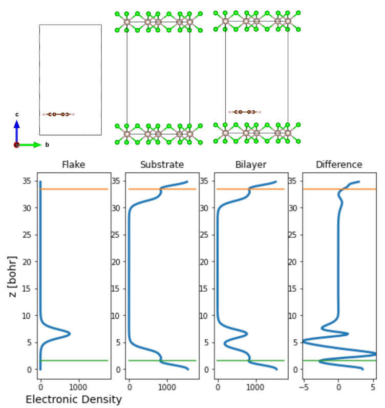
Once we obtain the optimized ionic positions of the interface, we calculate the charge density of each component of the MINT calculation, i.e., the substrate, the flake, and the interface, separately.
Fig. 2 Side view of the Graphene/α-RuCl3 interface and the corresponding electronic charge density. The difference is the difference between the charge density of the interface and its individual components, i.e., Difference = Bilayer - Flake - Substrate
Once the electronic density is obtained, one can plot the variation of the electronic charge density along the z-axis as shown above. The integral of the charge density yields the charge transfer between the substrate and the flake. At this point, the user needs to determine up to which the z-coordinate the charge transfer occurs — we suggest this to be taken to be the point where there is a minima in the charge density plots, as indicated by the green and orange lines above.
After the integration of the charge density up to the green line, we obtain the charge transfer to the α-RuCl3 layer to be 0.0096 e-/C atom. We then scale this value to the transfer expected for a full graphene layer L by multiplying by N(L)/N(C), the ratio of the (incommensurate) number of carbon atoms expected for a full graphene layer N(L) and the number in each cluster N(C), which is N(L)/N(C)=5.7. Therefore, for this particular example of 14 C-site graphene flake, the charge transfer is about 5.472% which is a value comparable to that obtained in the referenced manuscript.
Shifting the flake position:
Next, to further improve convergence with flake size, it is useful to repeat the above step, shifting the flake position on the substrate along the x-y plane, relaxing the ionic positions for each shifted flake, and finally taking the average of the charge transfer from several different flake positions. This allows for sampling all possible registries between the two monolayers, which is particularly important for small flake sizes. We leave this step to the user.
Change the flake size:
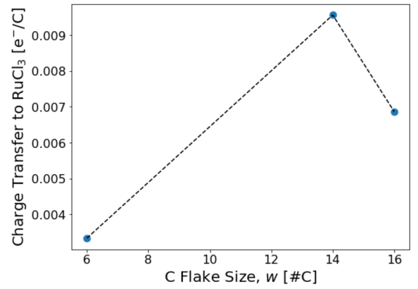
Finally, we vary the flake size to obtain the asymptotic limit of infinite flake size. For demonstration purposes, here we plot results for graphene flakes with 6 C atoms, 14 C atoms, and 16 C atoms. One can see that the charge transfer increases as the flake size increases initially. The fluctuation in the charge transfer as one goes from 14 to 16 C atom sites shows the importance of shifting the flake position on the substrate and taking an average of the charge transfer.
Once the charge transfer is sampled properly for each flake size and this calculation is repeated for several increasing flake sizes, one should get the result presented in the paper: E. Gerber et al. Phys. Rev. Lett. 124, 106804 (2020).
Nearsightedness of electronic matter ensures that, sufficiently far from the boundary of the flake, both materials behave just as they would for a truly infinite interface. Moreover, as the flake size increases, it eventually samples all possible registries with the other material. Appropriate finite-size scaling of thermodynamically intrinsic quantities then enables extraction of the behavior of the infinite interface.
Fig. 3 Charge transfer from the graphene to α-RuCl3, for one graphene flake position at each graphene flake size.
Below we present a python script in text format which in the future will also be hosted on our website as a Jupyter notebook. This script directly generates Fig. 3 of this tutorial.
# Electron density reading code adapted from JDFTx tutorial
# https://jdftx.org/Outputs.html
import numpy as np
import re
import matplotlib.pyplot as plt

# The user sets the following variables
#############################################################################
MINTpath = "../RUNS"  # Folder that contains the flakeDirs
nSubsLayers = 1                         # Number of substrate layers
flakeSizes = [6,14,16]                  # Number of atoms of interest (e.g. C for Graphene/RuCl3) per flake
flakeDirs = ["/6Site","/14Site","/16Site"] # Names of dirs in MINTpath, must match length of flakeSizes
shiftDirs = ["/shift000"] #,"/shift025","/shift050","/shift075"] # sub dirs for different flake displacement/orientations
# Make sure that shiftDirs is the union of the set of sub dir names over all flakeDirs

# Mark True if your spin up and spin down electron densities are split into two separate files
#    Also make sure to edit "nfile_up" and "nfile_dn"
spinPolar = True #False

outfile = "/totalE.out"       # All .out files must have this name
nfile = "/system.n"           # All .n files must have this name
nfile_up = "/system.n_up"     # All .n_up files must have this name (only need if spinPolar = True)
nfile_dn = "/system.n_dn"     # All .n_dn files must have this name (only need if spinPolar = True)
latfile = "/system.lattice"   # All .lattice files must have this name
ionposfile = "/system.ionpos" # All .ionpos files must have this name
# each MINTpath/flakeDir/shiftDir has these 3 folders for the full bilayer, isolated flake, and isolated substrate
#
BL_dir = "/bilayer"               # /directory for the interface
Flake_dir = "/isolated_flake"     # /directory for the isolated flake
Subs_dir = "/isolated_substrate"  # /directory for the isolated substrate

# Interface cutoff ranges:
# You will almost certainly have to change these for your system
# The interface btw the flake and the substrate is defined as the place where the total
#   electron density takes a minimum btw the two layers
# These four variables determine the bounds where the code will look for those interfaces
# units = fraction of unit cell height
lowerInterfaceBotGuess = 0.00
lowerInterfaceTopGuess = 0.05
upperInterfaceBotGuess = 0.95
upperInterfaceTopGuess = 1.00

# Plotting Labels
R_name = 'C'           # Name of the atomic species you report charge transfer in (e.g. R_name='C' -> dQ = 0.1 e-/C)
Subs_name = 'RuCl$_3$' # Name of the periodic substrate material
Flake_name = 'C'       # Name of the flake material

# Plots: Axis Label, Tick Font Size, Figure Size
fs = 20
fs_tick = 16
figsize = (8*0.8,6*0.8)
############################################################################

# Total electron density files
outfilename_tot = BL_dir+outfile         #'/Bilayer/totalE.out'
densityfilename_tot = BL_dir+nfile             #'/Bilayer/totalE.n'
densityfilename_tot_up = BL_dir+nfile_up       #'/Bilayer/totalE.n'
densityfilename_tot_dn = BL_dir+nfile_dn       #'/Bilayer/totalE.n'
# Flake Electron Density files
outfilename_flake = Flake_dir+outfile    #'/isolated_flake/totalE.out'
densityfilename_flake = Flake_dir+nfile        #'/isolated_flake/totalE.n'
densityfilename_flake_up = Flake_dir+nfile_up  #'/isolated_flake/totalE.n'
densityfilename_flake_dn = Flake_dir+nfile_dn  #'/isolated_flake/totalE.n'
# Substrate Electron Density files
outfilename_subs = Subs_dir+outfile      #'/isolated_substrate/totalE.out'
densityfilename_subs = Subs_dir+nfile          #'/isolated_substrate/totalE.n'
densityfilename_subs_up = Subs_dir+nfile_up    #'/isolated_substrate/totalE.n'
densityfilename_subs_dn = Subs_dir+nfile_dn    #'/isolated_substrate/totalE.n'

# return a list of all lines in filename with pattern
def grep(pattern, filename):
    retval = []
    foundPattern = False
    file = open(filename, "r")
    for line in file:
        if re.search(pattern, line):
            retval.append(line)
            foundPattern = True
    if not foundPattern:
        print("grep failed to find:", pattern, "in", filename)
        print("returning an empty list")
    return retval

def finalFreeEnergy(filename):
    return float(grep("F =",filename)[0].split()[2])

def get_ionpos_ionsp(path2file):
    ionspecies = []
    ionpos = []
    with open(path2file,'r') as file:
        # Skip the comment line at the top of the file
        line = file.readline()
        # record ionspecies, and lattice coordinate
        while line:
            line = file.readline()
            line_text = line.split()
            if len(line_text) > 0:
                if line_text[0] == "ion":
                    ionspecies.append(line_text[1])
                    ionpos.append([float(x) for x in line_text[2:5]])
    return ionpos,ionspecies

def get_LatticeMatrix(path2file):
    LatticeMatrix = []
    with open(path2file,'r') as file:
        # skip the first two lines
        #line = file.readline()
        line = file.readline()
        # get the contents as a list of lines
        contents = file.readlines()
        LM = [line.split()[:3] for line in contents]
        LatticeMatrix = np.array([ [float(i) for i in lm] for lm in LM ])
    return LatticeMatrix

# Looks for the minima in the Bilayer Electron density
# to determine where the RS flake ends and the TMD substrate begins
# z_min and z_max are initial guesses
def get_flake_range(n_BL,a,b,c,d):
    z_bot = n_BL.index(min(n_BL[a:b]))
    z_top = n_BL.index(min(n_BL[c:d]))
    return z_bot,z_top

# returns the total electron transfer onto the flake
def get_tot_dQ(diff,flake_bot,flake_top,dV):
    # Sum together the charge transfer from the average value bins
    tot_dQ = np.sum(diff[flake_bot:flake_top]) * dV
    #print("tot_dQ_naive =",tot_dQ)
    return tot_dQ

def get_CT(path,nSubsLayers,debug=False):
    LM = get_LatticeMatrix(path+BL_dir+latfile)
    ionpos,ionsp = get_ionpos_ionsp(path+BL_dir+ionposfile)
    a,b,c = LM.T
    cs = np.cross(a,b)/np.linalg.norm(np.cross(a,b)) # orthogonal to a and b
    Lz = np.dot(c,cs)  # bohr , for plotting purposes
    ionpos = np.matmul(ionpos,np.transpose(LM))
    NR = ionsp.count(str(ionsp[0]))
    NT = ionsp.count(str(ionsp[NR]))
    Y1z = float(np.dot(ionpos[NR+NT  ],cs)) % Lz
    Y2z = float(np.dot(ionpos[NR+NT+1],cs)) % Lz
    R1z = float(np.dot(ionpos[0],cs)) % Lz
    R2z = float(np.dot(ionpos[1],cs)) % Lz
    X1z = float(np.dot(ionpos[-1],cs)) % Lz
    X2z = float(np.dot(ionpos[-2],cs)) % Lz
    atomPlanes = [0.0,Y1z,R1z,X1z,X2z,R2z,Y2z]

    if spinPolar:
        n_tot_up = np.fromfile(path+densityfilename_tot_up,   # read from binary file
                  dtype=np.float64)      # as 64-bit (double-precision) floats
        #n = swapbytes(n)                # uncomment on big-endian machines; data is always stored litte-endian
        n_tot_dn = np.fromfile(path+densityfilename_tot_dn,   # read from binary file
                  dtype=np.float64)      # as 64-bit (double-precision) floats
        #n = swapbytes(n)                # uncomment on big-endian machines; data is always stored litte-endian
        n_tot = n_tot_up + n_tot_dn

        n_flake_up = np.fromfile(path+densityfilename_flake_up,   # read from binary file
                  dtype=np.float64)      # as 64-bit (double-precision) floats
        #n = swapbytes(n)                # uncomment on big-endian machines; data is always stored litte-endian
        n_flake_dn = np.fromfile(path+densityfilename_flake_dn,   # read from binary file
                  dtype=np.float64)      # as 64-bit (double-precision) floats
        #n = swapbytes(n)                # uncomment on big-endian machines; data is always stored litte-endian
        n_flake = n_flake_up + n_flake_dn

        n_subs_up = np.fromfile(path+densityfilename_subs_up,   # read from binary file
                  dtype=np.float64)      # as 64-bit (double-precision) floats
        #n = swapbytes(n)                # uncomment on big-endian machines; data is always stored litte-endian
        n_subs_dn = np.fromfile(path+densityfilename_subs_dn,   # read from binary file
                  dtype=np.float64)      # as 64-bit (double-precision) floats
        #n = swapbytes(n)                # uncomment on big-endian machines; data is always stored litte-endian
        n_subs = n_subs_up + n_subs_dn
    else:
        n_tot = np.fromfile(path+densityfilename_tot,   # read from binary file
                  dtype=np.float64)      # as 64-bit (double-precision) floats
        #n = swapbytes(n)                # uncomment on big-endian machines; data is always stored litte-endian
        n_flake = np.fromfile(path+densityfilename_flake,   # read from binary file
                  dtype=np.float64)      # as 64-bit (double-precision) floats
        #n = swapbytes(n)                # uncomment on big-endian machines; data is always stored litte-endian

        n_subs = np.fromfile(path+densityfilename_subs,   # read from binary file
                  dtype=np.float64)      # as 64-bit (double-precision) floats
    #n = swapbytes(n)                # uncomment on big-endian machines; data is always stored litte-endian
    ns = [n_tot,n_flake,n_subs]
    ofs = [outfilename_tot,outfilename_flake,outfilename_subs]

    n = n_tot
    outfilename = outfilename_tot
    #look for the first instance of the following in the output file
    #unit cell volume =
    #Chosen fftbox size, =
    S = []
    V = 0
    flag = 0
    with open(path+outfilename,'r') as file:
        line = file.readline()
        #print(line)
        while line:
            line = file.readline()
            contents = line.split()
            #
            if len(contents) > 0:
                if contents[0] == "unit":
                    V = float(contents[4])
                    flag += 1
                elif contents[0] == "Chosen":
                    S = [int(contents[6]),int(contents[7]),int(contents[8])]
                    flag += 1

            if flag >= 2:
                break
    dV = V / np.prod(S)

    # Total Bilayer electron density
    n_tot_slices = []
    for z in range(S[2]):
        nz = n_tot.reshape(S)[:,:,z]
        # Sum up the electron density
        # choose a xy slice slice of the electron density
        slicedensity = np.sum(nz)
        # add it to an array for plotting
        n_tot_slices.append(slicedensity)

    # Sum of isolated_flake and isolated_substrate electron densities
    n_flake_slices = []
    n_subs_slices = []
    n_sum_slices = []
    for z in range(S[2]):
        nz_flake = n_flake.reshape(S)[:,:,z]
        nz_subs  = n_subs.reshape(S)[:,:,z]
        # Sum up the electron density
        # choose a xy slice slice of the electron density
        density_flake = np.sum(nz_flake)
        density_subs = np.sum(nz_subs)
        # add it to an array for plotting
        n_flake_slices.append(density_flake)
        n_subs_slices.append(density_subs)
        n_sum_slices.append(density_flake+density_subs)

    # Average charge difference as a function of z
    diff = [n_tot_slices[i]-n_sum_slices[i] for i in range(S[2])]

    # Interface cutoffs are the minima of the total electron density in
    #  the ranges specified by the user
    a = int(lowerInterfaceBotGuess * len(n_tot_slices))
    b = int(lowerInterfaceTopGuess * len(n_tot_slices))
    c = int(upperInterfaceBotGuess * len(n_tot_slices))
    d = int(upperInterfaceTopGuess * len(n_tot_slices))
    flake_bot,flake_top = get_flake_range(n_tot_slices,a,b,c,d)

    if debug:
        zbot = flake_bot*Lz/S[2]
        ztop = flake_top*Lz/S[2]
        z_plot = np.arange(0,Lz,Lz/S[2])

        fig, axes = plt.subplots(nrows=1, ncols=4, figsize=(8, 5))
        titles = ["Flake","Substrate","Bilayer","Difference"]
        n_data = [n_flake_slices,n_subs_slices,n_tot_slices,diff]
        axes[0].set_xlabel("Electronic Density",fontsize=14)
        axes[0].set_ylabel("z [bohr]",fontsize=14)
        axes[3].set_xlim([np.min(diff), np.max(diff)])
        for i in range(4):
            axes[i].plot(n_data[i],z_plot,linewidth=3)
            axes[i].set_title(titles[i])
            axes[i].plot((-5,1750),(ztop,ztop))
            axes[i].plot((-5,1750),(zbot,zbot))
        #fig.tight_layout()
        plt.show()

    # Sum up the charge difference on the flake
    return get_tot_dQ(diff,flake_bot,flake_top,dV)

def get_BE(path):
    E_bl  = finalFreeEnergy(path+BL_dir+outfile)
    E_rs  = finalFreeEnergy(path+Flake_dir+outfile)
    E_tmd = finalFreeEnergy(path+Subs_dir+outfile)
    return E_bl - (E_rs + E_tmd)

print("""Use the plots below to tune lowerInterfaceBotGuess, lowerInterfaceTopGuess,
         upperInterfaceBotGuess, and upperInterfaceTopGuess""")
print("Green Line  = Lower Material Interface")
print("Organe Line = Upper Material Interface")

flag = True # for plotting one debug plot
CTs = [] # Charge Transfers
BEs = [] # Binding Energies
for flakeDir in flakeDirs:
    CTs_flake = []
    BEs_flake = []
    for shiftDir in shiftDirs:
        path = MINTpath+flakeDir+shiftDir
        # Not all flake dirs have all the shiftDirs, account for this
        try:
            CT = get_CT(path,nSubsLayers,debug=flag)
            CTs_flake.append(CT)
            BE = get_BE(path)
            BEs_flake.append(BE)
        except:
            print("Warning: Couldn't compute either CT or BE in", path)
        if flag:
            flag = False
    CTs.append(CTs_flake)
    BEs.append(BEs_flake)

print("")
print("Raw Charge Transfers:")
print(CTs)

# Plot wrt inverse flake size and fit line to the converging datapoints
# The converged charge transfer will be the y-intercept
inv_flakeSizes = 1.0/np.array(flakeSizes)

# Plot the charge transfer v.s. Flake Size
CT_perR = [ [-1*np.array(CTs[i])/flakeSizes[i]] for i in range(len(flakeSizes))]
avgCT_perR = [np.mean(ctf) for ctf in CT_perR]
maxCT_perR = [np.max(ctf)-np.mean(ctf) for ctf in CT_perR]
minCT_perR = [np.mean(ctf)-np.min(ctf) for ctf in CT_perR]
print("Averaged Charge Transfers per "+R_name+":")
print(avgCT_perR)
print("Upper and Lower Confidence:")
print("maxCT_perR-maxCT_perR =", maxCT_perR)
print("avgCT_perR-minCT_perR =", minCT_perR)
# Extract Bulk Charge Transfer from linear fit
dataCut = -3 # only linfit to the last "this many" points
p_linfit,p_cov = np.polyfit(inv_flakeSizes[dataCut:],avgCT_perR[dataCut:], 1,cov=True)
p = np.poly1d(p_linfit)
print("Bulk Charge Transfer =", p_linfit[1], u"\u00B1" , np.sqrt(p_cov[1][1]), "electrons")


# PLOT: Charge Transfers v.s. Flake Size
plt.figure(figsize=figsize)
plt.scatter(flakeSizes,avgCT_perR,s=80)
plt.errorbar(flakeSizes,avgCT_perR, yerr=[minCT_perR,maxCT_perR], fmt='k--')
plt.xlabel(Flake_name+' Strip Size, $w$ [#'+R_name+']',fontsize=fs)
plt.ylabel('Charge Transfer to '+Subs_name+' [e$^{-}$/'+R_name+']',fontsize=fs)
plt.xticks(fontsize=fs_tick, rotation=0)
plt.yticks(fontsize=fs_tick, rotation=0)
plt.show()


# PLOT: Charge Transfers v.s. Inverse Flake Size
#print("p_linfit =", p_linfit)
plt.figure(figsize=figsize)
plt.scatter(inv_flakeSizes,avgCT_perR,s=80)
# uncomment below to plot linear fit to the data in the "dQ v.s. inverse flake size" plot
#plt.plot([0,inv_flakeSizes[dataCut]],[p(0),p(inv_flakeSizes[dataCut])],c='black',linestyle='--')
plt.errorbar(inv_flakeSizes,avgCT_perR, yerr=[minCT_perR,maxCT_perR], fmt='k--')
plt.xlabel(Flake_name+' Strip Inverse Size, $w^{-1}$ [#'+R_name+'$^{-1}$]',fontsize=fs)
plt.ylabel('Charge Transfer to '+Subs_name+' [e$^{-}$/'+R_name+']',fontsize=fs)
#plt.xlim((0,0.275))
#plt.ylim((0.15,0.22))
plt.xticks(fontsize=fs_tick, rotation=0)
plt.yticks(fontsize=fs_tick, rotation=0)
plt.show()


BE_perR = [ [np.array(BEs[i])/flakeSizes[i]] for i in range(len(flakeSizes))]
avgBE_perR = [np.mean(ctf) for ctf in BE_perR]
maxBE_perR = [np.max(ctf)-np.mean(ctf) for ctf in BE_perR]
minBE_perR = [np.mean(ctf)-np.min(ctf) for ctf in BE_perR]
print("Averaged Interlayer Binding Energies per "+R_name+":")
print(avgBE_perR)
print("Upper and Lower Confidence:")
print("maxBE_perR-avgBE_perR =", maxBE_perR)
print("avgBE_perR-minBE_perR =", minBE_perR)
# Extract Bulk Binding Energies from linear fit
dataCut = -3 # only linfit to the last "this many" points
p_linfit,p_cov = np.polyfit(inv_flakeSizes[dataCut:],avgBE_perR[dataCut:], 1,cov=True)
p = np.poly1d(p_linfit)
print("Bulk Interlayer Binding Energy =", p_linfit[1]*27.2114, u"\u00B1" , np.sqrt(p_cov[1][1])*27.2114, "[eV]")

# PLOT: Binding Energies v.s. Flake Size
plt.figure(figsize=figsize)
plt.scatter(flakeSizes,avgBE_perR,s=80)
plt.errorbar(flakeSizes,avgBE_perR, yerr=[minBE_perR,maxBE_perR], fmt='k--')
plt.xlabel(Flake_name+' Strip Size [#'+R_name+']',fontsize=fs)
plt.ylabel('Interlayer B.E. [Hartree] [Hartree]',fontsize=fs)
plt.show()


# PLOT: Binding Energies v.s. Inverse Flake Size
#print("p_linfit =", p_linfit)
plt.figure(figsize=figsize)
plt.scatter(inv_flakeSizes,avgBE_perR,s=80)
# uncomment below to plot linear fit to the data in the "BE v.s. inverse flake size" plot
#plt.plot([0,inv_flakeSizes[dataCut]],[p(0),p(inv_flakeSizes[dataCut])])
plt.errorbar(inv_flakeSizes,avgBE_perR, yerr=[minBE_perR,maxBE_perR], fmt='k--')
plt.xlabel(Flake_name+' Strip Inverse Size [#'+R_name+'$^{-1}$]',fontsize=fs)
plt.ylabel('Interlayer B.E. [Hartree]',fontsize=fs)
plt.show()
The SciServer PARADIM Data Collective (PDC) Cloud is a collaborative research platform for large-scale data-driven science. SciServer includes tools and services to enable researchers to cope with Terabytes or Petabytes of scientific data without needing to download any large datasets. PARADIM users can run density functional theory (DFT) computational simulations and analyze microscopy data via inbuilt Jupyter notebook recipes. Focus of this tutorial is to show how users can login to the SciServer computing environment and launch Jupyter notebooks. For users new to Jupyter notebooks, this tutorial will show you how to create and test your first notebook. Through a series of notebook examples available on SciServer, you can then explore the capabilities of Jupyter notebooks with particular emphasis on topic relevant to PARADIM’s materials research.
How to Login to SciServer
In this tutorial you will learn how to access the PDC Cloud through an internet browser, how to create a new account, and how to gain access to specific PARADIM and SciServer resources.
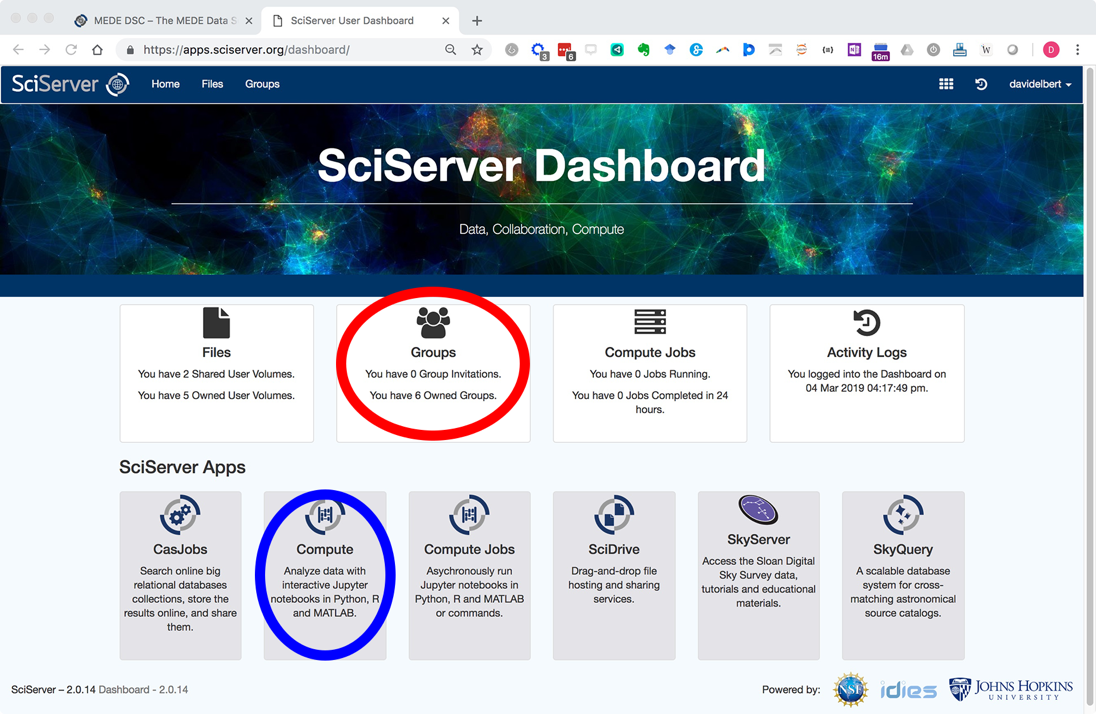
Click login and create a new account. Once logged in you will be navigated with the following Dashboard page:
Email pdc@jhu.edu to be added to the PARADIM user group and gain access to PARADIM specific resources.
You will receive a reply email within 24 hours inviting you to the PARADIM group. The next time you are login after being added to PARADIM group, your SciServer Dashboard will list the invitation in the “Groups” app (circled in red in the screenshot above).
Click “Groups” and accept the invitation.
How to Create and Launch a Container
Login to your SciServer account and start the Compute app (note that “Compute” and “Compute Jobs” are different and you need to open the “Compute”, circled in blue in the screenshot below)
In Compute, use the green button to Create a computing container.
Be sure to:
a. type in a name for your container
b. select the “PARADIM” Compute Image from the drop-down menu
c. check the “PARADIM Data Collective” volume to add it to your container
In a few seconds you will return to the “Compute” screen and you can see your running container.
Once your container is made, click the container to open a new browser tab accessing your compute container (If you are returning to a stopped container, you will have to click the green arrowhead to restart it).
The container mounts into a new browser tab showing the mounted volumes (paradim_data, storage, and temporary). The storage and temporary volumes are for your personal work. They will be available in any other SciServer container you make (they go with your account). The paradim_data storage is for data or work you want available to the whole PARADIM group.
Your storage volume is only 10 GB but is backed up and is permanent. Your temporary volume is part of 80 TB of storage shared between users. Temporary storage has no guarantee of long-term storage but can be used for weeks or even months at a time. You will be warned before it is cleaned up and given time to move anything you have stored there. The paradim_data volume is about 300 TB storage for sharing materials data. This is where experiment results will be shared.
How to Open a Notebook
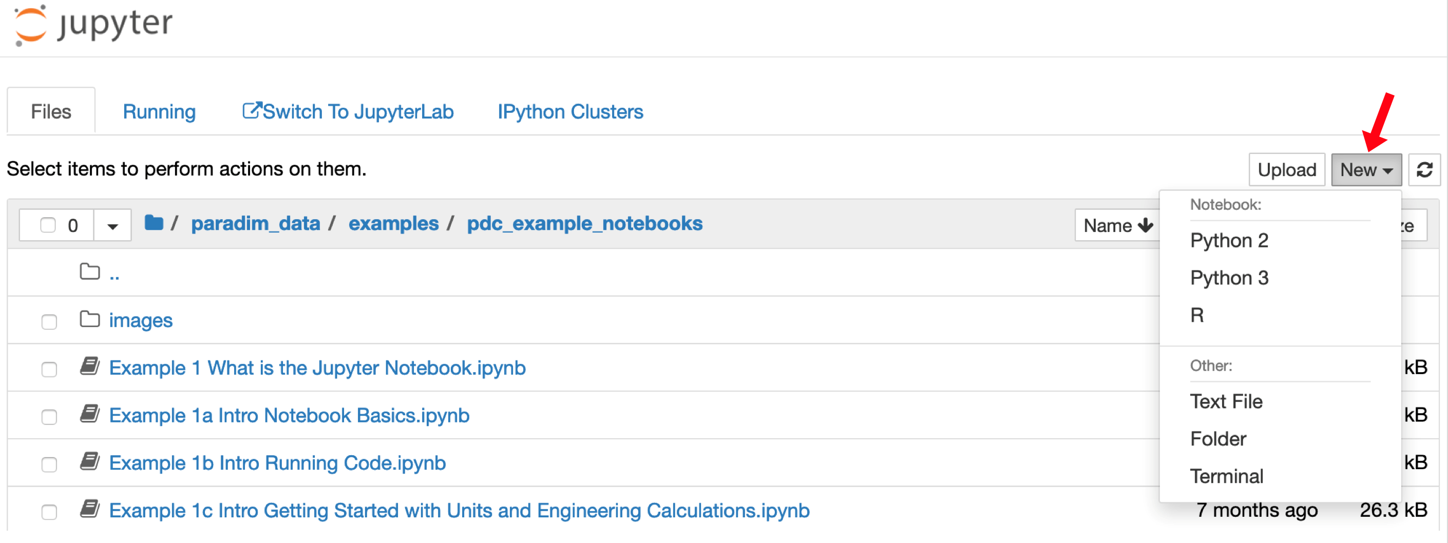
You can now make a notebook. To make a new notebook use the “New” menu on the right-hand side of the browser as shown here:
Choose “Python 3” and a new browser tab will open with a blank notebook.
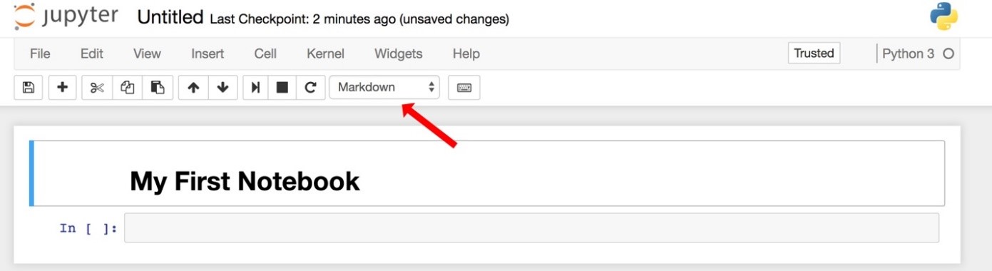
In the first cell type “# My First Notebook” (without the quotes)
Change the cell type to “markdown” and hit shift-enter.
Your notebook will look like this (the red arrow shows you the drop-down menu to make the cell "markdown" instead of code):
Notice that the kernel is Python 3 (shown on the right side) and that there are tools and menus you can look through and use.
Enter some Python code in the second cell and execute it.
Try 1+1 or try print ("All I dream about is reciprocal space.")
Save your notebook and continue following the tutorial to explore a range of SciServer notebook examples.
Please contact David Elbert (elbert@jhu.edu) or Nick Carey (ncarey4@jhu.edu) for any questions related to SciServer.
Your First SciServer Tutorial
Go back to the “Home” tab by clicking on the “Jupyter” logo, browse to the paradim_data volume and locate the “example>pdc_example_notebooks” folder. Open it.
Open the “ReadMePlease.ipynb” notebook for basic information about the example notebooks. Everything in the examples directory is read-only. If you want your own copies of the notebooks to play with, follow the directions in ReadMePlease.ipynd to copy the example notebooks to your own, persistent storage. Explore the Jupyter window’s menu bars and tools. These include editing tools and the ability to change or restart the computational kernel.
Close the notebook by using the File>Close and Halt in the Jupyter menubar.
Open “Example 1a Intro Notebook Basics". This notebook is a general overview of using Jupyter. If you’re new to Jupyter, read through the notebook and follow examples to edit cells and make menu choices.
Open “Example 1b Intro Running Code” to learn how to execute cells and run active code. Double-click your cursor into the first code cell (it has a gray background and the python code “a = 10”. Shift-enter to execute the cell. Execute the next cell (Shift-enter) to use the Python print statement to print back the value of a. Work through the other cells in Example 1b to get a feel for mixing execution and text in a notebook.
Go back to the “Home” tab and go to the Jupyter tab labeled “Running.” There you will find what notebooks and terminals you have open and running. You can go back to them by clicking on them or you can shut them down here. N.B. if you shutdown a notebook from this tab you don’t know what was saved. This is a really useful tab to get back to something that you left running the last time you were on the Data Science Cloud (DSC).
Example Notebook Tutorials Available on SciServer Once you have followed the above steps successfully the system is now ready for you to explore some further notebook tutorials,
Open the Example 5 notebook. Click in each cell to see the markdown (formatted text cells) and execute the calculations from top to bottom. There are four important things to learn in this notebook:
a. Jupyter has two modes: command and edit. Command mode is for moving around the notebook while edit mode lets you modify the contents of the cells. Esc puts you in command mode. Esc-enter puts you back in edit mode once you click into a cell.
b. You manually pick if a cell is code (executable) or markdown (formatted text). There is a drop-down menu to do (you can pick up key-stroke shortcuts later, but command mode M changes a cell to markdown and command mode Y changes it to code)
c. Cells need to be executed when you finish with your input. That means markdown (text) cells, too. Execute any cell with shift-enter.
d. You can use these notebooks to combine complex formatting, materials calculations, and something like a scanned image to fully investigate problems.
Open the Example 4 notebook. N.B. This notebook requires an updated key from the Materials Project. Go to https://www.materialsproject.org/ and login to the dashboard to get an API key. To use the Materials Project APIs, you need to get a new key every day.
a. Replace the API key in quotes of the first code cell in the Example 4 notebook with a fresh key.
b. Execute the cells in order to retrieve and display data from the Materials Project. The Materials Project is a data repository that has already calculated a range of properties for common materials. You can pull information directly into your notebooks to avoid duplicating that effort.
Open the Example 6 notebook. This notebook takes advantage of the preloaded Mantid environment in the MEDE-DSC. Mantid is a data analysis and visualization package created for neutron and muon scattering results from beamlines.
a. Read the text and execute the code in sequence. This notebook reads in a neutron data file from the ISIS Neutron Source Facility near Oxford.
b. Using Mantid calls, the cells plot the raw data as well as showing a smoothing function.
Mantid is the analysis package of choice at the Spallation Neutron Source (SNS) at Oak Ridge.
Jupyter Keyboard Shortcuts
Frequently used: Esc-goes to Command Mode where arrow keys let you navigate Enter-goes to edit mode where you can type in cells
In Command Mode: A-inserts new cell above B-inserts new cell below M-changes current cell to Markdown Y-changes current cell to code DD-(hit D twice) deletes the current cell Shift-Tab- will show the Docstring for code object you just typed ?-Typing ? before a command and evaluating it will show the Docstring Ctrl+Shift+hyphen will split the current cell into two at your cursor Esc+F to find and replace in code Esc+O to toggle cell output
Selecting Multiple Cells: Shift-J or Shift-down- selects the next cell down Shift-K or Shift-up selects the next cell above Shift-M merges selected cells
You can delete/copy/cut/paste multiply selected cells
Multicursor support like Sublime. Click and drag mouse while holding down Alt.
Additional Resources and References
Graphing Tools
matplotlib is the de-facto standard. It’s activated with %matplotlib inline - Here’s a Dataquest Matplotlib Tutorial. Inline it can be a little slow because it is rendered on the server-side, but it’s easy and well known.
Seaborn is built over matplotlib and makes building more attractive plots easier. Just by importing Seaborn, your matplotlib plots are made ‘prettier’ without any code modification.
mpld3 provides an alternative renderer (using d3) for matplotlib code. Quite nice, though incomplete.
bokeh is a better option for building interactive plots.
plot.ly can generate nice plots - this used to be a paid service only but was recently open sourced.
Altair is a relatively new declarative visualization library for Python. It’s easy to use and makes great looking plots, however the ability to customize those plots is not nearly as powerful as in matplotlib.
Further Readings
Numerical Python: A Practical Techniques Approach for Industry, Robert Johansson, 2015, available online through JHU Libraries
Python: Pocket Primer, Oswald Campesato, 2012, available online through JHU Libraries
Data Wrangling with Python, Jacqueline Kazil and Katherine Jarmul,